GEN13
GEN13 — Stores a polynomial whose coefficients derive from the Chebyshev polynomials of the first kind.
Description
Uses Chebyshev coefficients to generate stored polynomial functions which, under waveshaping, can be used to split a sinusoid into harmonic partials having a pre-definable spectrum.
Initialization
size -- number of points in the table. Must be a power of 2 or a power-of-2 plus 1 (see f statement). The normal value is power-of-2 plus 1.
xint -- provides the left and right values [-xint, +xint] of the x interval over which the polynomial is to be drawn. These subroutines both call GEN03 to draw their functions; the p5 value here is therefor expanded to a negative-positive p5, p6 pair before GEN03 is actually called. The normal value is 1.
xamp -- amplitude scaling factor of the sinusoid input that is expected to produce the following spectrum.
h0, h1, h2, etc. -- relative strength of partials 0 (DC), 1 (fundamental), 2 ... that will result when a sinusoid of amplitude
xamp * int(size/2)/xint
is waveshaped using this function table. These values thus describe a frequency spectrum associated with a particular factor xamp of the input signal.
GEN13 is the function generator normally employed in standard waveshaping. It stores a polynomial whose coefficients derive from the Chebyshev polynomials of the first kind, so that a driving sinusoid of strength xamp will exhibit the specified spectrum at output. Note that the evolution of this spectrum is generally not linear with varying xamp. However, it is bandlimited (the only partials to appear will be those specified at generation time); and the partials will tend to occur and to develop in ascending order (the lower partials dominating at low xamp, and the spectral richness increasing for higher values of xamp). A negative hn value implies a 180 degree phase shift of that partial; the requested full-amplitude spectrum will not be affected by this shift, although the evolution of several of its component partials may be. The pattern +,+,-,-,+,+,... for h0,h1,h2... will minimize the normalization problem for low xamp values (see above), but does not necessarily provide the smoothest pattern of evolution.
Examples
Here is an example of the GEN13 generator. It uses the file gen13.csd.
Example 1107. Example of the GEN13 generator.
See the sections Real-time Audio and Command Line Flags for more information on using command line flags.
<CsoundSynthesizer>
<CsOptions>
; Select audio/midi flags here according to platform
-odac  ;;;realtime audio out
;-iadc    ;;;uncomment -iadc if realtime audio input is needed too
; For Non-realtime ouput leave only the line below:
; -o gen13.wav -W ;;; for file output any platform
</CsOptions>
<CsInstruments>

sr = 44100
ksmps = 32
nchnls = 2
0dbfs  = 1
;example by Russell Pinkston - Univ. of Texas  (but slightly modified)

gisine   ftgen 0, 0, 16384, 10, 1							;sine wave

instr   1

ihertz = cpspch(p4)
ipkamp = p5
iwsfn  = p6										;waveshaping function
inmfn  = p7										;normalization function
agate   linen  1, .01, p3, .1            					 	;overall amp envelope
kctrl   linen  .99, 2, p3, 2								;waveshaping index control
aindex  poscil kctrl/2, ihertz, gisine							;sine wave to be distorted
asignal tablei .5+aindex, iwsfn, 1							;waveshaping
knormal tablei kctrl, inmfn, 1								;amplitude normalization
asig    =      asignal*knormal*ipkamp*agate
        outs   asig, asig

endin
</CsInstruments>
<CsScore>
; This proves the statement in Dodge (p. 147) that Chebyshev polynomials
; of order K have "only the kth harmonic." This is only true when the
; waveshaping index is at the maximum - i.e., when the entire transfer
; function is being accessed. RP.
;--------------------------------------------------------------------------------------------------------------------------------------------
; quasi sawtooth transfer function:
;		 h0   h1   h2   h3   h4   h5   h6    h7   h8   h9   h10   h11 	h12   h13    h14    h15    h16    h17    h18    h19    h20
f1 0 513 13 1 1  0   100  -50  -33   25   20 -16.7 -14.2 12.5 11.1 -10  -9.09  8.333  7.69  -7.14  -6.67  6.25	  5.88	-5.55  -5.26    5
f2 0 257 4 1 1	 ; normalizing function with midpoint bipolar offset

;	st	dur	pch	amp	wsfn	nmfn
i1      0       4      6.00    .7 	 1	 2
i1      4       .      7.00    .
i1      8       .      8.00    .
;--------------------------------------------------------------------------------------------------------------------------------------------
; quasi square wave transfer function:
;		 h0   h1   h2   h3   h4   h5   h6    h7   h8   h9   h10   h11 	h12   h13    h14    h15    h16    h17    h18    h19
f3 0 513 13 1 1  0   100   0   -33   0    20   0   -14.2  0   11.1   0  -9.09	 0   7.69     0    -6.67    0    5.88     0    -5.26
f4 0 257 4 3 1	 ; normalizing function with midpoint bipolar offset

;	st	dur	pch	amp	wsfn	nmfn
i1      16       4     6.00     .7	 3	 4
i1      20       .     7.00     .
i1      24       .     8.00     .
;--------------------------------------------------------------------------------------------------------------------------------------------
; quasi triangle wave transfer function:
;		 h0   h1   h2   h3   h4   h5   h6    h7   h8   h9   h10   h11 	h12   h13    h14    h15    h16    h17    h18    h19
f5 0 513 13 1 1  0   100   0  -11.11 0    4    0   -2.04  0   1.23  0   -.826	0    .59      0    -.444    0    .346     0   -.277
f6 0 257 4 5 1	 ; normalizing function with midpoint bipolar offset
;	st	dur	pch	amp	wsfn	nmfn
i1      32       4     6.00     .7	 5	 6
i1      36       .     7.00     .
i1      40       .     8.00     .
;--------------------------------------------------------------------------------------------------------------------------------------------
; transfer function1:  h0 h1 h2 h3 h4 h5 h6 h7 h8 h9 h10 h11 h12 h13 h14 h15 h16
f7 0 513 13 1 1        0  1 -.8 0 .6  0  0  0 .4  0  0   0   0   .1 -.2 -.3  .5
f8 0 257 4 7 1	       ; normalizing function with midpoint bipolar offset
;	st	dur	pch	amp	wsfn	nmfn
i1      48       4     5.00     .7	 7	 8
i1      52       .     6.00     .
i1      56       .     7.00     .
;--------------------------------------------------------------------------------------------------------------------------------------------
;=========================================================================;
; This demonstrates the use of high partials, sometimes without a         ;
; fundamental, to get quasi-inharmonic spectra from waveshaping.          ;
;=========================================================================;
; transfer function2:  h0 h1 h2 h3 h4 h5 h6 h7 h8 h9 h10 h11 h12 h13 h14 h15 h16
f9 0 513 13 1 1        0  0  0 -.1  0 .3  0 -.5 0 .7  0 -.9  0   1   0  -1   0
f10 0 257 4 9 1	       ; normalizing function with midpoint bipolar offset
;	st	dur	pch	amp	wsfn	nmfn
i1      64       4       5.00   .7	 9	10
i1      68       .       6.00    .
i1      72       .       7.00    .
;--------------------------------------------------------------------------------------------------------------------------------------------
; transfer function3: h0   h1   h2   h3   h4   h5   h6    h7   h8   h9   h10   h11 	h12   h13    h14    h15    h16    h17    h18    h19    h17   h18   h19   h20
f11 0 513 13 1 1      0    0    0    0    0    0    0     -1   0    1     0     0       -.1    0     .1      0     -.2    .3      0     -.7     0    .2     0    -.1
f12 0 257 4 11 1      ; normalizing function with midpoint bipolar offset

;	st	dur	pch	amp	wsfn	nmfn
i1      80       4     5.00     .7	 11	12
i1      84       .     5.06     .
i1      88       .     6.00     .
;--------------------------------------------------------------------------------------------------------------------------------------------
;=========================================================================;
; split a sinusoid into 3 odd-harmonic partials of relative strength 5:3:1
;=========================================================================;
;--------------------------------------------------------------------------------------------------------------------------------------------
; transfer function4: h0   h1   h2   h3   h4   h5
f13 0 513 13 1 1      0    5    0    3    0    1
f14 0 257 4 13 1      ; normalizing function with midpoint bipolar offset

;	st	dur	pch	amp	wsfn	nmfn
i1      96      4     5.00     .7	 13	14
i1      100     .     5.06     .
i1      104     .     6.00     .
e
</CsScore>
</CsoundSynthesizer>
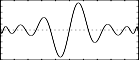
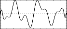
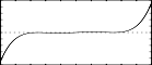
These are the diagrams of the waveforms of the GEN13 routines, as used in the example:
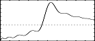
f1 0 513 13 1 1 0 100 -50 -33 25 20 -16.7 -14.2 12.5 11.1 -10 -9.09 8.333 7.69 -7.14 -6.67 6.25 5.88 -5.55 -5.26 5 - quasi sawtooth transfer function
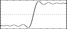
f3 0 513 13 1 1 0 100 0 -33 0 20 0 -14.2 0 11.1 0 -9.09 0 7.69 0 -6.67 0 5.88 0 -5.26 - quasi square wave transfer function
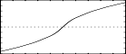
f5 0 513 13 1 1 0 100 0 -11.11 0 4 0 -2.04 0 1.23 0 -.826 0 .59 0 -.444 0 .346 0 -.277 - quasi triangle wave transfer function
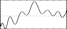
f7 0 513 13 1 1 0 1 -.8 0 .6 0 0 0 .4 0 0 0 0 .1 -.2 -.3 .5 - transfer function 1
f9 0 513 13 1 1 0 0 0 -.1 0 .3 0 -.5 0 .7 0 -.9 0 1 0 -1 0 - transfer function 2
f11 0 513 13 1 1 0 0 0 0 0 0 0 -1 0 1 0 0 -.1 0 .1 0 -.2 .3 0 -.7 0 .2 0 -.1 - transfer function 3
f13 0 513 13 1 1 0 5 0 3 0 1 - split a sinusoid into 3 odd-harmonic partials of relative strength 5:3:1
See Also
Information about the Chebyshev polynomials on Wikipedia: http://en.wikipedia.org/wiki/Chebyshev_polynomials